What Is a Signal? Time Domain vs Frequency Domain Explained for Telecom
Updated: May 7

A signal is one of the most fundamental ideas in telecommunications. Every phone call, video stream, WhatsApp message, 5G data session, satellite link, fiber broadband connection, Wi-Fi packet, and IPTV stream depends on signals. Yet the word “signal” is often used casually, as if it only means “network strength” on a mobile phone.
In engineering, a signal means something much deeper.
A signal is a physical quantity that changes in a way that carries information. That quantity may be voltage on a copper cable, electromagnetic field strength in free space, light intensity inside an optical fiber, acoustic pressure in air, or even a sequence of digital samples inside a processor.
When you speak into a smartphone, your voice creates pressure variations in air. A microphone converts those pressure variations into an electrical signal. That electrical signal is sampled, compressed, encoded, modulated, transmitted as radio waves, received by a base station, processed through the mobile core, routed through packet networks, and eventually reconstructed as sound at the other end.
At every stage, engineers ask questions like:
What does the signal look like over time?
How fast does it change?
How much bandwidth does it occupy?
How much noise has corrupted it?
Can it pass through this channel without distortion?
Can we compress it, filter it, amplify it, or recover it?
How much data can it carry?
To answer these questions, telecom engineers use two essential views of a signal: the time domain and the frequency domain.
The time domain shows how a signal changes with time. The frequency domain shows what frequencies are present inside that signal. These are not two different signals. They are two different ways of looking at the same signal.
A beginner may think the time-domain waveform is the “real” signal and the frequency domain is just a mathematical trick. In practical telecom engineering, that is not true. The frequency-domain view is just as real and often more useful. Spectrum planning, LTE resource blocks, 5G numerology, OFDM subcarriers, fiber dispersion, RF filters, antenna design, equalization, channel estimation, and noise analysis all depend heavily on frequency-domain thinking.
This article explains what a signal is from first principles, then gradually builds toward engineering-level understanding. We will move from intuition to equations, from simple waveforms to real telecom systems, and from textbook definitions to practical design trade-offs.

What Is a Signal?
A signal is a measurable physical or mathematical quantity that varies with one or more independent variables and carries information.
In most telecom systems, the independent variable is time. So we often write a signal as:

Here:
(x) is the signal value.
(t) is time.
(x(t)) means “the value of the signal at time (t).
For example, if (x(t)) represents microphone voltage, then (x(0.01)) might mean the voltage measured 10 milliseconds after recording began.
A signal can also vary with space:

This could represent an electromagnetic field at position (r) and time (t). In antenna engineering and radio propagation, signals are often functions of both space and time because the field changes as it travels.
In image processing, a signal may vary with two spatial coordinates:

In telecom, however, the most common signal model starts with time.
A useful way to understand a signal is this:
A signal is not the information itself, but the physical carrier of information.
The sentence “hello” is information. The sound pressure wave produced by your mouth is a signal. The microphone voltage is another signal. The encoded binary stream is another signal. The modulated RF waveform is another signal. Each signal represents the same underlying information in a different physical or mathematical form.
This distinction matters because telecom systems do not transmit abstract information directly. They transmit physical signals through imperfect channels.
A channel may be:
Air between a smartphone and a cell tower.
Optical fiber between cities.
Coaxial cable in a broadband network.
Twisted-pair copper in DSL.
Microwave links between towers.
Satellite links through atmosphere and space.
PCB traces inside telecom equipment.
Each channel affects signals differently. A wireless channel introduces fading, interference, Doppler shift, path loss, and multipath. An optical fiber introduces attenuation, chromatic dispersion, nonlinear effects, and amplifier noise. A copper channel introduces resistance, capacitance, crosstalk, and electromagnetic interference.
The signal must be designed so that information survives the channel.
That is why telecom engineering is not only about “sending data.” It is about shaping, encoding, transmitting, detecting, and recovering signals under real-world constraints.

Signals vs Data: A Critical Difference
Many people use “signal” and “data” interchangeably, but in telecom engineering they are different.
Data is the message or content.A signal is the physical or mathematical representation used to carry that data.
For example, suppose you send the text message:
“OK”
In binary using ASCII, “O” and “K” can be represented as:
O = 01001111
K = 01001011
The data is the bit sequence:
0100111101001011
But those bits cannot travel through air by themselves. A phone must map them into a waveform. In a wireless system, that may involve modulation such as QPSK, 16-QAM, 64-QAM, or 256-QAM. The resulting signal is a continuous-time electromagnetic wave.
In fiber optics, the same data may become pulses of light. In Ethernet over copper, it may become voltage levels on twisted-pair wires. In a processor, it may exist as digital logic levels.
This separation helps explain why the same data can be transported using different physical technologies. A YouTube video can travel through fiber, Wi-Fi, LTE, 5G, Ethernet, submarine cables, and data center switches. The data remains logically the same, but the signal representation changes many times along the path.
This is also why telecom systems use layered architectures. The application layer cares about data. The physical layer cares about signals.
At the physical layer, questions become very concrete:
Can this waveform fit inside the allocated bandwidth?
Can the receiver distinguish one symbol from another?
Is the signal strong enough compared to noise?
Will the amplifier distort it?
Will the filter remove important components?
Will multipath cause inter-symbol interference?
Will the optical pulse spread too much before reaching the receiver?
These are signal questions, not just data questions.

Analog and Digital Signals
Signals are often classified as analog or digital, but this classification can be misunderstood.
An analog signal varies continuously in time and amplitude. A classic example is
microphone voltage:
At any time (t), the voltage can theoretically take any value within a range.
A digital signal, in the physical sense, is usually a waveform that represents discrete values. For example, a logic signal may use approximately 0 V for binary 0 and 1 V for binary 1.
But here is the important engineering detail:
All real physical signals are analog at the lowest physical level.
Even a “digital” signal on a circuit board is a voltage waveform with finite rise time, ringing, noise, reflections, and distortion. It is interpreted as digital because the receiver maps voltage ranges to discrete symbols.
For example:
A voltage below 0.3 V may be interpreted as binary 0.
A voltage above 0.7 V may be interpreted as binary 1.
Values in between may be uncertain.
In telecom, digital communication does not mean the transmitted waveform is a perfect square wave. Modern LTE and 5G systems transmit carefully shaped analog RF waveforms that represent digital symbols.
A 5G base station transmitting 256-QAM is sending an analog electromagnetic waveform. The receiver samples and processes that waveform to estimate which digital symbols were sent.
So “digital communication” means the information is represented using discrete symbols, not that the physical signal is magically immune to analog impairments.
This distinction is essential. Noise, interference, distortion, phase error, frequency offset, nonlinear amplification, and timing error all affect digital telecom systems because the physical signal is still analog.

Continuous-Time and Discrete-Time Signals
Another important classification is continuous-time versus discrete-time.
A continuous-time signal is defined for every instant of time:
A discrete-time signal is defined only at specific time instants:

Here:
n is an integer sample index.
x[n] means the n-th sample of the signal.
If a continuous-time signal x(t) is sampled every Tₛ seconds, the discrete-time signal is:

where:
(Tₛ) is the sampling period.
fₛ = 1/Tₛ is the sampling frequency.
For example, audio may be sampled at 48 kHz. That means:


In telecom receivers, RF signals are eventually converted down to baseband and sampled by analog-to-digital converters. Once sampled, digital signal processors operate on sequences such as:
x[0], x[1], x[2], . . .
This is where modern communication becomes heavily algorithmic. Equalization, filtering, synchronization, channel estimation, demodulation, decoding, beamforming, and interference cancellation are often performed digitally.
But sampling introduces its own constraints. If the sampling rate is too low, aliasing occurs. Frequencies that are too high appear falsely as lower frequencies. This is why anti-aliasing filters are required before analog-to-digital conversion.
The sampling theorem says that a band-limited signal with maximum frequency (B) can be perfectly reconstructed from samples if:
fₛ > 2B
The value (2B) is called the Nyquist rate.
In real systems, engineers usually sample above the theoretical minimum because filters are not ideal, clock jitter exists, and implementation margins are needed.

Deterministic and Random Signals
Some signals are deterministic. That means they can be described exactly by a mathematical expression.
For example:

where:
A is amplitude.
f is frequency.
ɸ is phase.
t is time.
If all parameters are known, the signal value can be predicted at any time.
But many telecom signals are random or stochastic. Voice, video, internet traffic, thermal noise, fading, interference, and user data are not perfectly predictable.
Random signals are described using statistical properties such as:
Mean
Variance
Power spectral density
Autocorrelation
Probability distribution
Signal-to-noise ratio
For example, thermal noise in a receiver is often modeled as additive white Gaussian noise, abbreviated AWGN. This means the noise is added to the signal, has a flat power spectral density over the bandwidth of interest, and has amplitude values following a Gaussian distribution.
A simple received signal model is:
y(t) = x(t) + n(t)
where:
y(t) is the received signal.
x(t) is the transmitted signal.
n(t) is noise.
In wireless systems, the channel may also scale and delay the signal:
y(t) = h(t) * x(t) + n(t)
Here:
h(t) is the channel impulse response.
* denotes convolution.
n(t) is noise.
This equation is extremely important. It says the received signal is not just a weaker copy of the transmitted signal. It is the transmitted signal filtered by the channel, then corrupted by noise.
In LTE and 5G, estimating h(t) or its frequency-domain equivalent is a major receiver task. Without channel estimation, the receiver cannot reliably recover the transmitted symbols.

The Time Domain: Seeing How a Signal Changes Over Time
The time domain is the most intuitive way to view a signal. It shows signal amplitude as a function of time.
For a voltage signal, the vertical axis may be volts and the horizontal axis may be seconds. For an optical signal, the vertical axis may represent optical power. For an acoustic signal, it may represent pressure variation.
A time-domain plot answers question like:
What is the signal value at a particular time?
How quickly does it rise or fall?
Does it contain pulses?
Does it repeat periodically?
Does it decay?
Does it have sudden transitions?
Is it noisy?
Is there delay between two signals?
Are symbols overlapping?
For example, a sinusoidal signal in the time domain can be written as:
The physical meaning of each variable matters:
A is amplitude.
f is frequency.
ɸ is phase.
t is time.
2𝜋f: angular frequency in radians per second.
The period T of the sinusoid is:
T = 1/f
If f = 1 kHz, then:
T = 1 ms
That means the waveform completes one full cycle every millisecond.
In telecom, time-domain thinking is critical for timing synchronization, symbol duration, pulse shaping, latency, propagation delay, guard intervals, cyclic prefixes, and transient behavior.
For example, in OFDM systems such as LTE and 5G, each OFDM symbol has a certain duration. If multipath delay spread is too large compared to the guard interval, symbols interfere with each other. This is a time-domain problem.
Similarly, when a fiber optic pulse travels through a long fiber, it may spread in time due to dispersion. If pulses spread too much, adjacent bits overlap. Again, this is a time-domain effect.

Time-Domain Parameters Engineers Care About
A beginner may look at a waveform and only notice its shape. Engineers extract specific parameters from it.
Amplitude
Amplitude represents the magnitude of the signal. For voltage, it is measured in volts. For current, amperes. For electric field strength, volts per meter. For optical power, watts or dBm.
Amplitude is related to power. For a voltage signal across resistance (R), average power is often:

where:
P is power.
Vᵣₘₛ is root-mean-square voltage.
R is resistance.
In RF systems, power is frequently expressed in dBm:

A signal power of 1 mW is 0 dBm. A signal power of 10 mW is 10 dBm. A signal power of 0.001 mW is -30 dBm.
Mobile receivers often work with extremely weak signals, sometimes below -100 dBm. That is less than a trillionth of a watt. Recovering information from such weak signals requires careful receiver design, low-noise amplification, filtering, synchronization, coding, and signal processing.
Period and Frequency
For periodic signals, the period is the time required for one cycle. Frequency is the number of cycles per second:
f = 1/T
In telecom, frequency determines where a signal sits in the spectrum. A 900 MHz cellular signal has a carrier oscillating 900 million times per second. But the useful information is usually not in the carrier alone. It is in how the carrier is modulated.
Phase
Phase describes where a waveform is in its cycle. Two sinusoids with the same frequency may be shifted relative to each other.
Phase is crucial in coherent communication systems. QPSK and QAM modulation encode information partly through phase. MIMO systems depend on phase relationships between antennas. Beamforming works by controlling phase and amplitude across antenna elements so signals combine constructively in desired directions.
Rise Time
Rise time measures how quickly a signal transitions from one level to another. In high-speed digital systems, fast rise times create high-frequency components. This affects electromagnetic compatibility, PCB design, cable behavior, and signal integrity.
A common mistake is assuming a digital signal with a low bit rate has no high-frequency content. In reality, sharp edges contain high-frequency components. That is why high-speed Ethernet, backplane links, and telecom hardware require careful impedance control and termination.
Delay
Delay is the time shift between cause and effect. In networks, delay affects latency. In signal processing, delay affects synchronization. In antenna arrays, delay and phase control beam direction.
Propagation delay depends on medium. In free space, electromagnetic waves travel at approximately:
c = 3×10⁸ m/s
In fiber, light travels slower, roughly:
v ≈ c/η
where η is the refractive index. For typical fiber, η is around 1.5, so speed is roughly 2×10⁸. That means light takes about 5 microseconds to travel 1 km in fiber.
This matters in long-haul networks, cloud gaming, financial trading networks, 5G fronthaul, and synchronization systems.

The Frequency Domain: Seeing What a Signal Is Made Of
The frequency domain shows how much of each frequency is present in a signal.
Instead of asking, “How does the signal change over time?” we ask:
Which frequencies does this signal contain?
How much power exists at each frequency?
What bandwidth does it occupy?
Where is the carrier?
Are there unwanted harmonics?
Is there interference nearby?
How does the channel affect different frequencies?
Can a filter separate this signal from others?
The key idea is that complex signals can be represented as combinations of sinusoids. A sinusoid is special because it is a pure frequency. Many signals that look complicated in time can be understood as a mixture of frequency components.
The mathematical tool that connects time and frequency is the Fourier transform.
For a continuous-time signal (x(t)), the Fourier transform is:

Here:
x(t) is the time-domain signal.
X(f) is the frequency-domain representation.
f is frequency in hertz.
j is the imaginary unit.
e⁻ʲ²ᵖⁱᶠᵗ represents a complex sinusoidal basis function.
The inverse Fourier transform is:

This means we can move from time domain to frequency domain and back without losing information, assuming mathematical conditions are satisfied.
For discrete-time sampled signals, engineers use the discrete Fourier transform, or DFT:

where:
x[n] is the discrete-time signal.
X[k] is the k-th frequency bin.
N is the number of samples.
n is the time sample index.
k is the frequency bin index.
The fast Fourier transform, or FFT, is an efficient algorithm for computing the DFT. FFTs are everywhere in telecom: spectrum analyzers, OFDM receivers, channel estimation, interference analysis, measurement equipment, and digital signal processors.

Why Frequency Domain Is Not Just “Theory”
The frequency domain is not an abstract classroom concept. It directly controls how telecom systems are planned and deployed.
Mobile operators buy spectrum licenses in frequency bands. For example, a network may operate in 700 MHz, 1800 MHz, 2300 MHz, 3500 MHz, or mmWave bands. Each band has different propagation characteristics, antenna requirements, bandwidth availability, and deployment cost.
A 700 MHz signal travels farther and penetrates buildings better than a 3500 MHz signal but usually has less available bandwidth. A 3500 MHz 5G signal can support wider channels and higher capacity, but coverage is more limited. mmWave can offer very large bandwidth but suffers from high path loss, blockage, and limited range.
These are frequency-domain realities.
Spectrum regulators allocate different frequency ranges for cellular, satellite, Wi-Fi, microwave backhaul, broadcasting, aviation, emergency services, radar, and other systems. Without frequency-domain planning, systems would interfere with each other.
In a real cellular network, engineers must manage:
Licensed spectrum blocks.
Channel bandwidth.
Adjacent-channel leakage.
Intermodulation products.
Spurious emissions.
Guard bands.
Duplex spacing.
Uplink and downlink separation.
Coexistence with other technologies.
Receiver blocking and selectivity.
All of these are frequency-domain engineering issues.
When a spectrum analyzer is connected to an RF system, it does not show packets or bits directly. It shows signal power versus frequency. Engineers use that view to detect interference, verify bandwidth, inspect emissions, check modulation quality, and diagnose faults.

Time Domain vs Frequency Domain: Two Views of the Same Signal
The time domain and frequency domain are complementary. Neither is “better” in every situation.
The time domain is better when analyzing:
Waveform shape.
Pulses.
Timing.
Delay.
Transients.
Symbol boundaries.
Jitter.
Rise time.
Time alignment.
Multipath delay spread.
The frequency domain is better when analyzing:
Bandwidth.
Spectrum occupancy.
Filtering.
Carrier frequency.
Harmonics.
Interference.
Noise distribution.
Channel frequency response.
Modulation spectra.
OFDM subcarriers.
A short pulse in time spreads widely in frequency. A pure sinusoid in time occupies one frequency. A sharp square wave has many harmonics. A slowly varying signal occupies lower frequencies. A rapidly changing signal needs higher bandwidth.
This leads to a deep engineering principle:
Time localization and frequency localization are connected by trade-off.
If a signal is very short in time, it cannot be extremely narrow in frequency. If a signal is very narrow in frequency, it must extend over a longer time. This principle appears in pulse shaping, OFDM design, radar, filter design, and spectral efficiency.
For example, in LTE and 5G, OFDM uses many narrow subcarriers. Narrow subcarriers are useful because each subcarrier experiences approximately flat fading. But narrow subcarriers require longer symbol duration. Longer symbols help with multipath robustness, but they also affect latency and sensitivity to phase noise and Doppler.
So, when telecom engineers choose subcarrier spacing, they are balancing time-domain and frequency-domain constraints.

Simple Example: A Pure Sine Wave
Consider:

In the time domain, this is a smooth repeating wave.
In the frequency domain, an ideal infinite-duration cosine has energy at two frequencies:
+f₀
and
-f₀
The negative frequency may seem strange at first. It comes from complex exponential representation. Using Euler’s formula:

A real cosine is made of two complex exponentials: one rotating positively and one rotating negatively.
In practical RF systems, engineers often use complex baseband representation, where negative frequencies become meaningful and useful. Instead of handling only real passband waveforms, we represent signals using in-phase and quadrature components:
s(t) = I(t) + jQ(t)
where:
I(t) is the in-phase component.
Q(t) is the quadrature component.
j represents a 90-degree phase shift.
This complex representation simplifies modulation, demodulation, filtering, and channel estimation. It is foundational in LTE, 5G, Wi-Fi, satellite communication, and software-defined radio.

Complex Signals and I/Q Representation
Modern telecom signals are usually described using I/Q samples. This is one of the concepts most beginner explanations skip, but it is essential for engineering-level understanding.
A passband RF signal can be written as:

where:
Xrf is the real transmitted RF waveform.
s(t) is the complex baseband signal.
f꜀ is the carrier frequency.
Re{⋅} means taking the real part.
The complex baseband signal is:
s(t) = I(t) + jQ(t)
Expanding gives:

This equation shows that a modulator uses two carrier waves:
A cosine carrier for the I component.
A sine carrier for the Q component.
They are 90 degrees apart, or in quadrature.
Why do this?
Because I/Q representation lets us control both amplitude and phase of the carrier. That allows modulation schemes like QPSK, 16-QAM, 64-QAM, and 256-QAM.
In QAM, each symbol corresponds to a point in the I/Q plane. The receiver estimates the received point and decides which symbol was transmitted. Noise and distortion move the point away from its ideal location. Engineers visualize this using constellation diagrams.
A clean constellation means good signal quality. A scattered constellation indicates noise, phase error, nonlinear distortion, interference, or synchronization problems.
In LTE and 5G, modulation order is adapted based on channel quality. A user near the tower with high signal-to-noise ratio may use 256-QAM. A cell-edge user with poor channel conditions may use QPSK. Higher-order modulation carries more bits per symbol but requires better signal quality.
This is a practical trade-off between data rate and reliability.

What Is Bandwidth?
Bandwidth is one of the most important signal concepts in telecom.
In simple terms, bandwidth is the range of frequencies occupied or required by a signal.
If a signal occupies frequencies from f₁ to f₂, its bandwidth is:
B = f₂ - f₁
For example, if a channel spans from 3.50 GHz to 3.60 GHz, its bandwidth is:
B = 3.60 GHz - 3.50 GHz = 100 MHz
But bandwidth has several meanings depending on context:
Signal Bandwidth
This is the actual frequency range occupied by the signal.
Channel Bandwidth
This is the allocated frequency range available for transmission.
Occupied Bandwidth
This is often defined as the bandwidth containing a certain percentage of total signal power, such as 99%.
Noise Bandwidth
This relates to how much noise power enters a receiver through a filter.
Coherence Bandwidth
This describes the frequency range over which a wireless channel response is approximately constant.
A crucial relationship in communication theory is Shannon capacity:
C = B log₂ (1+ SNR)
where:
C is channel capacity in bits per second.
B is bandwidth in hertz.
SNR is signal-to-noise ratio as a linear value, not dB.
This equation tells us that capacity increases linearly with bandwidth but logarithmically with SNR. Doubling bandwidth can roughly double capacity, but improving SNR gives diminishing returns.
This is why 5G systems seek wider bandwidths, especially in mid-band and mmWave spectrum. But wider bandwidth comes with practical challenges: more noise power, harder RF design, more ADC/DAC demand, higher processing load, and stricter linearity requirements.

Frequency, Wavelength, and Propagation
Frequency also determines wavelength:
λ = v/f
where:
λ is wavelength.
v is propagation speed.
f is frequency.
In free space:
λ = c/f
For a 900 MHz signal:

For a 3.5 GHz signal:

For a 28 GHz mmWave signal:

Wavelength affects antenna size, diffraction, penetration, scattering, and beamforming.
Lower-frequency signals have longer wavelengths. They generally diffract better around obstacles and penetrate buildings more effectively. Higher-frequency signals have shorter wavelengths, enabling compact antenna arrays and narrow beams, but they are more easily blocked and attenuated.
This is why low-band cellular spectrum is valuable for coverage, while mid-band and high-band spectrum are valuable for capacity.
A 700 MHz cell can cover a wide rural area. A 3.5 GHz 5G cell may provide high capacity in urban areas but needs denser site deployment. A 28 GHz mmWave cell may deliver very high throughput over short distances but requires line-of-sight or near-line-of-sight conditions.
This is not marketing. It is physics.

What Is Spectrum?
Spectrum is the frequency-domain real estate used by communication systems.
When people say “a telecom operator owns spectrum,” they mean the operator has rights to transmit in specific frequency ranges under regulatory conditions.
A spectrum block may be paired or unpaired.
In frequency division duplexing, or FDD, uplink and downlink use separate frequency bands. For example:
Uplink: user equipment to base station.
Downlink: base station to user equipment.
In time division duplexing, or TDD, uplink and downlink share the same frequency band but transmit at different times.
FDD has advantages when traffic is symmetric and paired spectrum is available. TDD is flexible because uplink and downlink ratios can be adjusted. Since modern networks often have more downlink traffic than uplink traffic, TDD is attractive for 5G mid-band deployments.
But TDD also introduces synchronization challenges. Neighboring cells must coordinate uplink and downlink timing to avoid interference. If one cell is transmitting downlink while another nearby cell is receiving uplink on the same frequency, severe interference can occur.
This is a system-level example of how time-domain and frequency-domain decisions interact.
Spectrum is limited. Demand is high. Therefore, modern telecom systems focus on spectral efficiency:
η = R/B
where:
η is spectral efficiency in bits/s/Hz.
R is data rate in bits per second.
B is bandwidth in hertz.
Higher spectral efficiency means more data transmitted per unit bandwidth. Techniques such as higher-order modulation, MIMO, beamforming, coding, scheduling, and interference coordination improve spectral efficiency.
But there are limits. Higher spectral efficiency usually requires better SNR, better channel conditions, more antennas, more processing, and tighter implementation quality.

Modulation: How Information Shapes a Signal
Modulation is the process of varying a carrier signal to represent information.
A carrier can be written as:

where:
(A꜀) is carrier amplitude.
(f꜀) is carrier frequency.
Information can be embedded by changing amplitude, frequency, or phase.
Amplitude Modulation
In amplitude modulation, the carrier amplitude varies according to the message:

where m(t) is the message signal.
Frequency Modulation
In frequency modulation, the instantaneous frequency changes according to the message.
Phase Modulation
In phase modulation, the carrier phase changes according to the message:

Digital modulation uses discrete symbol choices. For example, QPSK uses four possible phase states. 16-QAM uses 16 constellation points. 256-QAM uses 256 points.
If a modulation scheme has (M) symbols, each symbol carries log₂(M) bits.
So:
QPSK: (M=4), carries 2 bits/symbol.
16-QAM: (M=16), carries 4 bits/symbol.
64-QAM: (M=64), carries 6 bits/symbol.
256-QAM: (M=256), carries 8 bits/symbol.
But packing more points into the same constellation makes them closer together. The receiver needs higher SNR to distinguish them reliably.
This is why adaptive modulation is used. The system dynamically chooses modulation and coding based on channel quality.
In LTE and 5G, the network scheduler assigns modulation and coding schemes to users depending on radio conditions, interference, mobility, and quality feedback.

Baseband vs Passband Signals
A baseband signal is centered around 0 Hz. A passband signal is shifted to a higher carrier frequency.
For example, your data symbols may first exist as a baseband signal s(t). To transmit wirelessly, the signal is upconverted to RF:

At the receiver, the RF signal is downconverted back to baseband for processing.
Why not process everything directly at RF?
Because a 3.5 GHz RF signal oscillates billions of times per second. Directly processing that waveform digitally at the carrier frequency would be expensive and inefficient. Instead, RF front-end circuits shift the signal down to baseband or intermediate frequency, where ADCs and digital processors can handle it more practically.
A typical receiver chain includes:
Antenna.
RF filter.
Low-noise amplifier.
Mixer/downconverter.
Local oscillator.
Baseband filter.
ADC.
Digital signal processing.
The transmitter performs the reverse process:
Digital bits.
Coding and modulation.
Baseband waveform generation.
DAC.
Filtering.
Upconversion.
Power amplification.
Antenna transmission.
Baseband representation is one of the reasons software-defined radio is possible. Engineers can design modulation, filtering, synchronization, and demodulation algorithms in digital baseband while RF hardware handles frequency translation and amplification.

Fourier Transform Intuition: Why Complex Waveforms Contain Frequencies
A useful intuition is to imagine the Fourier transform as a frequency detector.
For each frequency (f), the Fourier transform compares the signal (x(t)) with a complex sinusoid at that frequency. If the signal contains that frequency strongly, the result is large. If it does not, the result is small.
The exponential term:

acts like a rotating reference wave. Multiplying the signal by this reference and integrating over time measures how much of that frequency exists in the signal.
This is closely related to how receivers work. A radio receiver mixes an incoming RF signal with a local oscillator. Mixing shifts frequencies. After filtering, the receiver extracts the desired band.
In other words, Fourier analysis is not disconnected from hardware. The same mathematical principle appears physically in mixers, filters, oscillators, and demodulators.
A pure sinusoid has a narrow frequency representation. A square wave has many harmonics because sharp transitions require high-frequency components. A pulse has broad spectrum because it changes quickly in time.
This matters in telecom because signals must fit inside assigned channels. If a signal has sharp transitions without pulse shaping, it spills energy into adjacent frequencies and interferes with neighboring channels.
Therefore, transmitters use pulse-shaping filters to control spectral spreading.

Pulse Shaping and Why Signals Cannot Change Instantly
In digital communication, symbols are transmitted one after another. A naive approach would send rectangular pulses. But rectangular pulses have poor spectral behavior.
A rectangular pulse in time has a sinc-shaped spectrum:

The sinc spectrum has sidelobes that extend far in frequency. Those sidelobes can cause adjacent-channel interference.
To reduce unwanted spectral leakage, systems use pulse shaping. A common pulse shape is the raised cosine filter. It controls bandwidth while reducing inter-symbol interference.
The raised cosine frequency response has a roll-off factor α, where:

The required bandwidth for symbol rate Rₛ is often:

for a baseband raised cosine response.
Here:
B is one-sided baseband bandwidth.
Rₛ is symbol rate.
α is roll-off factor.
A smaller roll-off uses less bandwidth but requires sharper filters and may be more sensitive to timing errors. A larger roll-off is easier to implement but consumes more spectrum.
This is a classic telecom trade-off: bandwidth efficiency versus implementation robustness.
Pulse shaping also affects peak-to-average power ratio, adjacent-channel leakage, receiver complexity, and timing recovery.
In LTE and 5G OFDM systems, pulse shaping is not used exactly the same way as in single-carrier systems, but spectral containment is still a major issue. OFDM subcarriers have sinc-like spectra, and windowing or filtering may be used to reduce out-of-band emissions.

Noise: The Unwanted Signal Always Present
No telecom signal travels alone. Noise is always present.
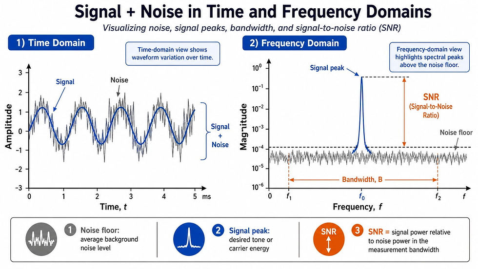
Thermal noise arises from random motion of electrons. Its available noise power over bandwidth (B) is:
N = kTB
where:
N is noise power in watts.
k is Boltzmann’s constant.
T is absolute temperature in kelvin.
B is bandwidth in hertz.
At room temperature, thermal noise density is approximately:
-174 dBm/Hz
Total noise power increases with bandwidth:

where:
B is bandwidth in hertz.
NF is receiver noise figure in dB.
This equation is extremely practical.
If a receiver bandwidth is 10 MHz:
10log₁₀(10⁷) = 70
Thermal noise over 10 MHz is:
-174 + 70 = -104 dBm
If receiver noise figure is 5 dB:
N = -99 dBm
This means widening bandwidth increases capacity potential but also admits more noise. A 100 MHz 5G channel has 10 dB more thermal noise than a 10 MHz channel, assuming the same noise figure.
Signal-to-noise ratio is:

In dB:

SNR affects modulation choice, coding rate, throughput, coverage, and error probability.
Channel Effects in the Time Domain
A telecom channel modifies the signal. In the time domain, a linear time-invariant channel can be described by its impulse response:
h(t)
If the transmitted signal is (x(t)), the received signal is:
y(t) = x(t) ∗ h(t)
Convolution means the received signal is a weighted combination of delayed versions of the transmitted signal.
In wireless communication, multipath occurs when the signal reaches the receiver through multiple paths due to reflection, diffraction, and scattering.
A simplified multipath channel is:

where:
ai is the complex gain of the (i)-th path.
𝜏i is the delay of the (i)-th path.
δ(t) is the impulse function.
L is the number of paths.
Then:

This means the receiver gets multiple delayed and scaled copies of the transmitted signal.
If delayed copies overlap with later symbols, inter-symb
ol interference occurs. This was a major problem in older single-carrier systems and remains important in many communication links.
OFDM handles multipath by adding a cyclic prefix. The cyclic prefix is a copy of the end of the OFDM symbol placed at the beginning. If the channel delay spread is shorter than the cyclic prefix, multipath interference can be converted into a simpler frequency-domain multiplication per subcarrier.
That design choice is one of the reasons OFDM became dominant in LTE, 5G, Wi-Fi, and broadband systems.

Channel Effects in the Frequency Domain
The frequency-domain version of the channel is called the channel frequency response:
H(f)
It is the Fourier transform of the impulse response h(t).
The time-domain convolution becomes multiplication in frequency:
Y(f) = X(f)H(f) + N(f)
This is one of the most powerful facts in signal processing.
Instead of dealing with convolution directly, engineers can analyze how each frequency component is scaled and phase-shifted by the channel.
If H(f) is flat across the signal bandwidth, all frequency components are affected similarly. This is called flat fading.
If H(f) varies significantly across the signal bandwidth, different frequencies experience different gains and phases. This is called frequency-selective fading.
Frequency-selective fading can severely distort wideband signals. But OFDM solves this by dividing a wideband channel into many narrowband subcarriers. Each subcarrier sees approximately flat fading, making equalization simpler.
For an OFDM subcarrier (k), a simplified model is:

The receiver estimates Hₖ using pilot or reference signals, then equalizes:

This equation is simple, but real implementation is not. If (H_k) is very small due to deep fading, dividing by it amplifies noise. More advanced equalizers use minimum mean square error techniques to balance channel inversion and noise enhancement.
This is an engineering detail many beginner explanations miss: equalization is not just “undoing the channel.” It involves trade-offs under noise and imperfect channel estimation.

OFDM: Where Time and Frequency Meet in LTE and 5G
Orthogonal Frequency Division Multiplexing, or OFDM, is one of the best real-world examples of time-domain and frequency-domain thinking working together.
OFDM divides a high-rate data stream across many narrow subcarriers. Each subcarrier carries lower-rate symbols. The subcarriers overlap in frequency but remain mathematically orthogonal.
The baseband OFDM signal can be written as:

where:
N is the number of subcarriers.
Xₖ is the data symbol on subcarrier (k).
Δf is subcarrier spacing.
t is time.
Orthogonality requires that subcarrier spacing is related to useful symbol duration:

where:
Δf is subcarrier spacing.
Tᵤ is useful OFDM symbol duration.
In LTE, normal subcarrier spacing is 15 kHz. The useful symbol duration is approximately:

A cyclic prefix is added to handle multipath.
5G NR supports multiple subcarrier spacings:
15 kHz
30 kHz
60 kHz
120 kHz
240 kHz in some contexts
This is called flexible numerology.
Why does 5G need different subcarrier spacings?
Because different frequency bands and use cases have different constraints.
At lower frequencies, Doppler shift and phase noise are less severe, and larger cells may have larger delay spreads. Smaller subcarrier spacing and longer symbols can be useful.
At mmWave frequencies, phase noise and Doppler effects become more challenging, and cells are smaller. Wider subcarrier spacing and shorter symbols become more practical.
This is not arbitrary. It reflects the time-frequency trade-off.

LTE Example: Resource Blocks and Frequency-Domain Scheduling
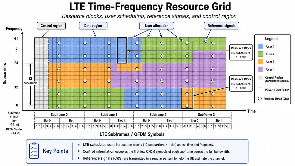
LTE uses OFDM in the downlink. The system organizes time and frequency resources into a grid.
A basic LTE resource block occupies:
12 subcarriers.
Each subcarrier is 15 kHz.
Total frequency width: 180 kHz.
12 × 15 kHz = 180 kHz
In time, resources are organized into slots and subframes. A 1 ms subframe contains multiple OFDM symbols depending on cyclic prefix configuration.
The scheduler decides which users get which resource blocks at which times. A user with good channel quality on certain frequencies may be assigned those resource blocks. Another user may be assigned different blocks.
This is frequency-domain scheduling.
Because wireless channels vary across frequency, one user may have a strong channel on one part of the band while another user has a better channel elsewhere. The base station can exploit this variation to improve total system throughput.
This is called multi-user diversity.
LTE receivers also measure reference signals to estimate channel quality. The user equipment reports channel quality indicators, which help the base station choose modulation, coding, and resource allocation.
So, in LTE, the signal is not just “sent over a frequency.” It is continuously managed across a time-frequency grid with feedback, scheduling, coding, and adaptation.
5G Example: Flexible Numerology and Real Deployment Trade-Offs
5G NR extends the OFDM idea with flexible numerology. The subcarrier spacing is:

where:
μ is the numerology index.
μ = 0 gives 15 kHz.
μ = 1 gives 30 kHz.
μ = 2 gives 60 kHz.
μ = 3 gives 120 kHz.
As subcarrier spacing increases, OFDM symbol duration decreases.
This affects latency, Doppler tolerance, phase noise robustness, cyclic prefix duration, and scheduling granularity.
For example, a 30 kHz subcarrier spacing has half the useful symbol duration of 15 kHz. That can reduce time latency and improve robustness to certain impairments, but it also changes the relative cyclic prefix behavior and resource grid structure.
5G deployments often use 30 kHz subcarrier spacing in mid-band spectrum such as around 3.5 GHz. mmWave deployments may use 120 kHz because high carrier frequencies face stronger phase noise and Doppler challenges, and wide bandwidths are common.
The key point is that 5G signal design is not one-size-fits-all. It adapts the time-frequency structure to deployment realities.
A rural low-band 5G cell, an urban 3.5 GHz macro cell, and an indoor mmWave small cell may all use different signal configurations because their channels and engineering constraints differ.

Fiber Optic Signals: Time, Frequency, and Dispersion
Telecom is not only wireless. Fiber optic networks also depend deeply on signal behavior.
In fiber systems, information is carried by light. A transmitter laser converts electrical data into optical signals. The receiver photodiode converts optical power back into electrical current.
At first glance, fiber may seem simpler than wireless because the signal is guided through a cable. But fiber has its own impairments.
One major impairment is attenuation. Optical power decreases with distance. Another is dispersion, where different parts of the signal travel at different speeds.
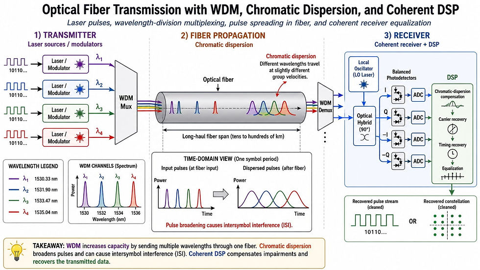
Chromatic dispersion occurs because different optical wavelengths propagate at slightly different velocities in fiber. This spreads pulses over time.
If a pulse starts narrow but becomes wider after traveling through fiber, it may overlap with neighboring pulses. This causes inter-symbol interference.
In frequency-domain terms, the fiber channel has a frequency-dependent phase response. That phase response translates into time-domain pulse spreading.
Long-haul optical systems use advanced modulation, coherent detection, digital signal processing, dispersion compensation, optical amplifiers, and wavelength division multiplexing.
Wavelength division multiplexing, or WDM, sends multiple optical carriers at different wavelengths through the same fiber. This is frequency-domain multiplexing in the optical domain.
Dense WDM systems can carry many channels, each at high data rates, over a single fiber pair. But channel spacing, laser linewidth, nonlinear effects, amplifier noise, and dispersion must be carefully managed.
So even in fiber, the question “what is a signal” leads directly to time-domain pulses, frequency-domain spectra, and system-level design.
ISP Networks: Signals Below the IP Layer
When people think about ISP networks, they often think about IP addresses, routing, DNS, and bandwidth plans. But below all of that, physical signals carry the packets.
A home fiber broadband connection may use passive optical network technology. Data is transmitted as optical signals between an optical line terminal at the provider side and optical network terminals at customer premises.
A cable broadband network uses RF signals over coaxial cable. DOCSIS systems allocate upstream and downstream channels in frequency. Cable modems tune to channels, measure SNR, handle modulation profiles, and deal with noise ingress.
DSL uses copper telephone lines. The line is divided into many frequency bins using discrete multitone modulation, which is similar in spirit to OFDM. Each tone can carry a different number of bits depending on channel quality.
Ethernet over twisted-pair copper also uses sophisticated signaling. High-speed Ethernet must deal with crosstalk, echo, attenuation, reflections, and equalization.
From the user’s perspective, the ISP sells “100 Mbps” or “1 Gbps.” From the physical-layer perspective, that service depends on signal bandwidth, modulation, coding, channel quality, noise, power levels, and error correction.
This is why two customers with the same package may experience different stability if the physical medium differs. A fiber link, a long copper DSL loop, and a noisy coax segment are not equal from a signal perspective.

Filters: Selecting What Matters and Rejecting What Does Not
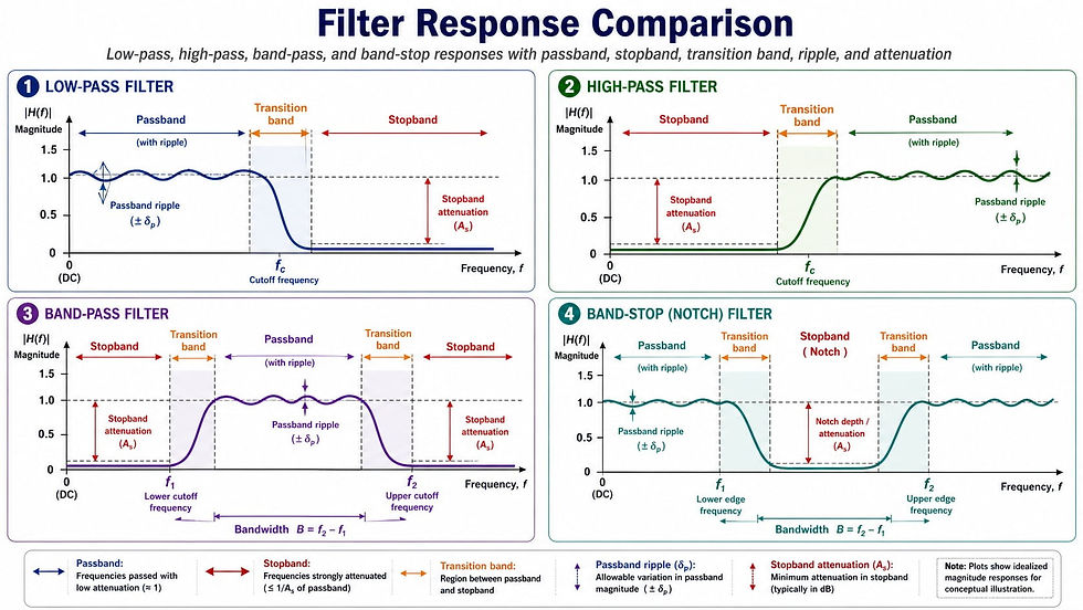
Filters are systems that modify signals based on frequency.
A low-pass filter passes low frequencies and attenuates high frequencies.
A high-pass filter passes high frequencies and attenuates low frequencies.
A band-pass filter passes a selected frequency band.
A band-stop filter rejects a selected frequency band.
In telecom, filters are everywhere:
RF front-end filters reject out-of-band interference.
Channel filters select desired communication channels.
Anti-aliasing filters protect ADCs.
Reconstruction filters smooth DAC outputs.
Duplexers separate transmit and receive bands.
Baseband filters shape pulses.
Optical filters select WDM channels.
A filter can be described by its impulse response h(t) in time domain or transfer function H(f) in frequency domain.
The input-output relation is:
y(t) = x(t) * h(t)
In frequency domain:
Y(f) = X(f)H(f)
This means filtering is convolution in time but multiplication in frequency.
Ideal filters are impossible. A perfect brick-wall filter would have an infinitely long impulse response. Real filters have transition bands, ripple, group delay variation, insertion loss, finite rejection, nonlinearities, and implementation cost.
Group delay is especially important. If different frequency components experience different delay, the signal waveform can distort. In communication systems, this can degrade error vector magnitude and increase bit errors.
Engineers must balance selectivity, insertion loss, group delay, cost, size, power consumption, and temperature stability.
Signal Power, SNR, SINR, and Link Budget
Telecom engineers rarely evaluate a signal alone. They evaluate it relative to noise and interference.
SNR compares signal power to noise power:
SNR = S/N
SINR compares signal power to noise plus interference:
SINR = S/(I+N)
where:
(S) is desired signal power.
(I) is interference power.
(N) is noise power.
In cellular networks, SINR is often more important than SNR because interference from neighboring cells and users can dominate thermal noise.
A simplified received power model is:
Pᵣ = Pₜ + Gₜ + Gᵣ - Lₚ - Lₛ
in dB units, where:
Pᵣ is received power.
Pₜ is transmit power.
Gₜ is transmit antenna gain.
Gᵣ is receive antenna gain.
Lₚ is path loss.
Lₛ represents additional losses such as cable loss, penetration loss, foliage loss, or body loss.
Path loss increases with distance and frequency. A common free-space path loss equation is:

when:
d is distance in kilometers.
f is frequency in MHz.
This equation shows why higher frequencies suffer greater free-space path loss for the same distance and antenna gains.
However, antenna aperture and array gain complicate real comparisons. Higher frequencies allow more antenna elements in the same physical area, enabling beamforming gain. This is one reason mmWave systems can work despite high path loss, although blockage and coverage remain major challenges.
A link budget combines all gains and losses to determine whether a communication link is feasible.

Interference: When Other Signals Become the Problem
Noise is random and unavoidable. Interference is usually caused by other transmitters, devices, or unwanted emissions.
Interference can occur in many forms:
Co-channel interference.
Adjacent-channel interference.
Intermodulation distortion.
Receiver blocking.
Spurious emissions.
Passive intermodulation.
Uplink interference from faulty devices.
External interference from non-telecom equipment.
In frequency domain, interference may appear as extra energy inside or near the desired channel. In time domain, it may appear as bursts, impulsive noise, or periodic disturbances.
Cellular networks are often interference-limited rather than noise-limited. This means increasing transmit power does not always solve the problem. If every cell increases power, interference also rises.
Network optimization involves controlling antenna tilt, transmit power, frequency reuse, scheduling, handovers, beamforming, and interference coordination.
In OFDM systems, narrowband interference may damage only certain subcarriers, while wideband interference affects many. The receiver may use coding and interleaving to recover from localized damage.
In fiber systems, interference may appear as crosstalk between wavelength channels, nonlinear mixing products, or amplifier noise accumulation.
In cable networks, ingress noise from poor shielding or faulty connectors can degrade upstream channels.
Understanding interference requires both time-domain and frequency-domain views. A spectrum analyzer may reveal where interference exists. A time-domain capture may reveal when it occurs.

Distortion and Nonlinearity
Real systems are not perfectly linear. Amplifiers, mixers, lasers, ADCs, DACs, and power amplifiers introduce distortion.
A linear system obeys superposition. If input x₁(t) produces output y₂(t), and input
x₁(t) produces output y₂(t), then input:
ax₁(t) + bx₂(t)
produces:
ay₁(t) + by₂(t)
Nonlinear systems violate this rule.
Power amplifiers are a major source of nonlinearity in wireless transmitters. If driven too hard, they distort the signal and create spectral regrowth. That means energy spreads into adjacent channels, potentially violating emission limits and interfering with other users.
OFDM signals have high peak-to-average power ratio, or PAPR. This means occasional peaks are much larger than average signal power. To avoid clipping those peaks, the power amplifier must operate with back-off, reducing power efficiency.
This is a major challenge in LTE and 5G base stations and user equipment.
The trade-off is clear:
More linear operation improves signal quality and reduces emissions.
But linear operation often reduces power efficiency.
Higher efficiency saves energy and heat but risks distortion.
Engineers measure modulation quality using error vector magnitude, or EVM. EVM measures the difference between ideal constellation points and received or transmitted points.
Lower EVM means cleaner modulation. Higher EVM may be caused by noise, phase error, IQ imbalance, nonlinear distortion, frequency offset, or filtering problems.

Time-Frequency Trade-Offs in Real Engineering
One of the most important lessons in signal engineering is that every design choice has trade-offs.
Short Symbols vs Long Symbols
Short symbols reduce latency and can improve tracking of fast channel changes. But they require larger bandwidth for the same pulse shape and may be more vulnerable to multipath delay spread.
Long symbols are more robust to delay spread and allow narrow subcarriers, but they may increase latency and become more sensitive to frequency offset or phase noise.
Narrowband vs Wideband
Narrowband signals are easier to process and may have better coverage due to lower noise bandwidth. Wideband signals support higher data rates and better time resolution but require more spectrum, higher sampling rates, and more complex RF hardware.
High Frequency vs Low Frequency
Low frequencies provide coverage and penetration. High frequencies provide bandwidth and compact antenna arrays but suffer from blockage and path loss.
High Modulation Order vs Robustness
256-QAM carries more bits per symbol than QPSK but requires much cleaner channel conditions.
Strong Filtering vs Signal Distortion
Sharp filters reduce adjacent-channel leakage but may introduce group delay distortion and implementation complexity.
High Transmit Power vs Interference and Battery Life
Higher transmit power improves link budget but increases interference, power consumption, heat, and regulatory constraints.
These trade-offs explain why real telecom systems are adaptive. A fixed design cannot perform optimally across all users, channels, mobility conditions, and deployment scenarios.

Sampling, ADCs, and Digital Signal Processing
Modern telecom systems depend on digital signal processing, but the physical world is analog. The bridge is the analog-to-digital converter.
An ADC samples and quantizes an analog signal.
Sampling converts continuous time into discrete time. Quantization converts continuous amplitude into discrete levels.
If an ADC has N bits, it has:
2ᴺ
quantization levels.
A 12-bit ADC has:
2¹² = 4096
levels.
Quantization introduces quantization noise. For an ideal ADC, signal-to-quantization-noise ratio is approximately:
SQNR ≈ 6.02N + 1.76 dB
for a full-scale sine wave.
Higher-resolution ADCs provide better dynamic range but may consume more power and be harder to operate at high sampling rates. Wideband 5G receivers need high-speed ADCs. Massive MIMO systems may need many ADC chains, making power consumption a major issue.
This is especially important in base stations, where dozens or hundreds of antenna elements may be used. Each receive chain may require filtering, amplification, mixing, sampling, and digital processing.
Engineers must balance:
Sampling rate.
Resolution.
Dynamic range.
Power consumption.
Cost.
Linearity.
Clock jitter.
Data converter architecture.
DSP workload.
Clock jitter is also critical. Timing uncertainty during sampling creates noise, especially for high-frequency signals. As carrier frequencies and bandwidths increase, clock quality becomes more important.

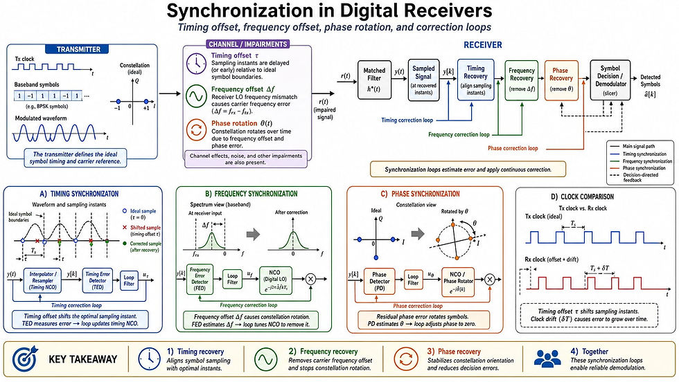
Frequency Offset, Phase Noise, and Synchronization
A receiver must align with the transmitter in time and frequency. Perfect alignment is impossible, so systems estimate and correct errors.
Frequency Offset
If the receiver local oscillator frequency differs from the transmitter carrier frequency, a frequency offset occurs.
If transmitted baseband signal is shifted by (\Delta f), the received signal may include a rotating phase term:

This rotation can destroy constellation accuracy if not corrected.
In OFDM, frequency offset is especially harmful because it breaks subcarrier orthogonality, causing inter-carrier interference.
Phase Noise
Oscillators are not perfect. Their phase fluctuates randomly over time. This is phase noise.
At high carrier frequencies, such as mmWave, phase noise becomes more challenging. Wider subcarrier spacing in 5G mmWave helps reduce sensitivity to phase noise.
Timing Synchronization
The receiver must know where symbols begin. If sampling happens at the wrong time, inter-symbol interference and detection errors increase.
In LTE and 5G, synchronization signals help user equipment detect and align with cells. Reference signals help estimate the channel and maintain coherent demodulation.
Synchronization is one of the hidden miracles of telecom. A phone moving through a city, surrounded by reflections and interference, must still lock onto a base station, estimate timing and frequency, track channel variations, and decode data reliably.
Signals in MIMO and Beamforming
Multiple-input multiple-output, or MIMO, uses multiple antennas at the transmitter, receiver, or both.
In MIMO, signals are not only functions of time and frequency. They also have a spatial dimension.
A simplified MIMO system can be written as:
y = Hx + n
where:
x is the transmitted signal vector.
y is the received signal vector.
H is the channel matrix.
n is noise vector.
Each element of H represents the channel between one transmit antenna and one receive antenna.
MIMO can be used for:
Spatial diversity.
Spatial multiplexing.
Beamforming.
Interference suppression.
Coverage improvement.
Capacity improvement.
Beamforming adjusts amplitude and phase across antenna elements so signals combine in desired directions.
For a uniform linear array, phase shifts between antenna elements steer the beam. If antenna spacing is d, wavelength is λ, and desired angle is θ, phase progression is related to:
Δϕ = 2πdsinθ/λ
This is why wavelength matters. At higher frequencies, wavelength is smaller, so many antenna elements can fit into compact arrays. That enables massive MIMO and narrow beams in 5G mid-band and mmWave systems.
But beamforming also requires accurate channel state information, calibration, and fast adaptation. Mobility, blockage, and hardware imperfections complicate real deployments.

Time Domain in Network Latency and Fronthaul
Signals also matter beyond the radio waveform. In telecom transport networks, timing and latency are engineering constraints.
5G radio access networks may use fronthaul links connecting radio units to distributed units. These links can carry digitized radio samples or processed splits depending on architecture.
If the functional split is close to the radio, fronthaul may require very high capacity and strict timing. Transport delay, jitter, and synchronization affect radio performance.
Timing synchronization is also essential for TDD networks. If neighboring base stations are not synchronized, uplink/downlink interference can occur.
Precision Time Protocol, GNSS timing, SyncE, and other timing systems help maintain network synchronization.
In packet networks, latency is not only propagation delay. It includes:
Serialization delay.
Queuing delay.
Processing delay.
Switching delay.
Routing path length.
Retransmission delay.
At the physical layer, signal propagation sets the lower bound. Fiber distance matters. A packet cannot travel faster than the signal carrying it.
This becomes important for ultra-low-latency applications, cloud gaming, industrial control, financial networks, and edge computing.

How Engineers Measure Signals
Telecom engineers use different instruments depending on the signal type and domain.
Oscilloscope
An oscilloscope shows time-domain waveforms. It is used for voltage signals, rise time, jitter, pulse shape, eye diagrams, and transient behavior.
Spectrum Analyzer
A spectrum analyzer shows power versus frequency. It is used for RF emissions, interference hunting, occupied bandwidth, harmonics, adjacent-channel leakage, and noise floor.
Vector Signal Analyzer
A vector signal analyzer captures I/Q data and analyzes modulation quality, constellation, EVM, frequency error, and channel behavior.
Network Analyzer
A vector network analyzer measures frequency response, reflection, transmission, impedance, and S-parameters.
Optical Spectrum Analyzer
Used in fiber networks to inspect optical wavelengths, WDM channels, optical signal-to-noise ratio, and spectral shape.
Protocol Analyzer
Although protocol analyzers operate above the physical waveform, they help connect signal problems to packet-level symptoms such as retransmissions, low throughput, or session drops.
A common engineering mistake is using only one view. For example, a network may show poor throughput. The cause may be RF interference, low SINR, bad modulation quality, packet loss, scheduling congestion, transport delay, or core network issues.
Good troubleshooting moves across layers and domains.

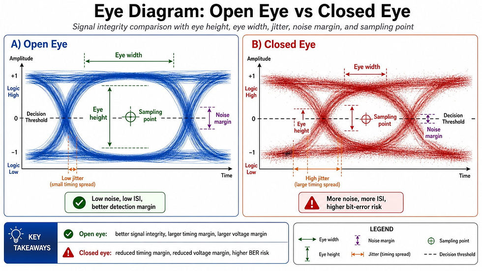
Eye Diagrams: Time-Domain View of Digital Signal Quality
An eye diagram overlays many bits or symbols on top of each other in time. It is commonly used in high-speed digital communication and optical systems.
A clean eye diagram has a wide eye opening. That means the receiver has margin to distinguish symbols despite noise and timing uncertainty.
A closed eye indicates problems such as:
Noise.
Jitter.
Inter-symbol interference.
Bandwidth limitation.
Reflections.
Dispersion.
Poor equalization.
Nonlinear distortion.
Eye height relates to noise margin. Eye width relates to timing margin.
In optical links, dispersion and noise can close the eye. In copper links, channel loss and reflections can close the eye. In high-speed serial links, equalization is used to reopen the eye.
Eye diagrams are powerful because they show time-domain signal integrity in a way directly related to receiver decisions.
Spectrograms: When Signals Change Over Time
A normal frequency-domain plot shows frequency content averaged over a time window. But many telecom signals change with time. For that, engineers use a spectrogram.
A spectrogram shows frequency versus time, with color or intensity representing power.
It answers:
Which frequencies are active at which times?
Is interference continuous or bursty?
Are frequency hops occurring?
Does a signal drift?
Are uplink bursts aligned correctly?
Is a radar pulse present?
Are TDD slots visible?
Mathematically, a spectrogram is based on the short-time Fourier transform:

where:
w(t−τ) is a window centered around time (\tau).
f is frequency.
X(τ,f) shows frequency content near time (\tau).
There is a trade-off between time resolution and frequency resolution. A short window gives good time resolution but poor frequency resolution. A long window gives good frequency resolution but poor time resolution.
This trade-off appears in spectrum monitoring, radar, wireless diagnostics, and signal classification.

Why a Signal Needs Both Energy and Structure
A signal must be strong enough, but strength alone is not enough.
A high-power distorted signal may be useless. A weak but clean signal may be recoverable with coding and processing. A signal with good average power may still fail if phase noise, interference, or timing errors are severe.
Telecom signal quality depends on structure:
Correct modulation.
Controlled spectrum.
Accurate timing.
Stable frequency.
Low distortion.
Sufficient SNR/SINR.
Manageable multipath.
Recoverable coding.
Proper synchronization.
Hardware linearity.
For example, two users may show similar received signal strength indicator, or RSSI, but very different throughput. Why? RSSI measures total received power, including interference and noise. A user with high RSSI but poor SINR may perform badly. Another user with lower RSSI but cleaner channel may achieve better data rates.
This is why modern systems use metrics such as RSRP, RSRQ, SINR, CQI, BLER, EVM, and throughput together.
A signal is not only “how loud” it is. It is how clean, structured, synchronized, and distinguishable it is.

Common Misconceptions About Signals
Misconception 1: A Digital Signal Is Just Ones and Zeros
At the information level, yes. At the physical level, no. Digital signals are analog waveforms interpreted as discrete values. Noise, distortion, bandwidth, and timing still matter.
Misconception 2: Higher Frequency Always Means Faster Internet
Higher frequency can provide access to wider bandwidth, but frequency itself does not guarantee speed. Throughput depends on bandwidth, SNR, modulation, MIMO, scheduling, backhaul, device capability, and network load.
Misconception 3: More Signal Bars Always Mean Better Performance
Signal bars are simplified indicators. They may not reflect interference, congestion, bandwidth, modulation, or network scheduling.
Misconception 4: Frequency Domain Is Only for RF Engineers
Frequency-domain thinking applies to audio, fiber, copper, wireless, filters, digital signal processing, data converters, and network diagnostics.
Misconception 5: OFDM Eliminates Multipath Completely
OFDM handles multipath efficiently when delay spread is within the cyclic prefix and channel estimation works well. Severe delay spread, high Doppler, phase noise, or poor synchronization can still degrade performance.
Misconception 6: More Bandwidth Has No Downside
More bandwidth increases potential capacity, but also increases noise power, hardware complexity, sampling rate, processing load, and spectrum cost.
Putting It All Together: A Smartphone 5G Download
Let us connect all concepts through a real example: a smartphone downloading data over 5G.
At the application layer, the phone requests data from a server. At the physical layer, the base station must transmit bits over a wireless channel.
The bits are encoded for error correction. They are mapped into modulation symbols such as QPSK, 16-QAM, 64-QAM, or 256-QAM. These symbols are placed into a time-frequency resource grid. OFDM converts frequency-domain subcarrier symbols into a time-domain waveform using an inverse FFT.
A cyclic prefix is added. The digital signal is converted to analog by a DAC. It is filtered, upconverted to RF, amplified, and transmitted through an antenna array.
The radio wave propagates through the environment. It reflects from buildings, diffracts around edges, scatters from objects, and experiences path loss. The phone receives multiple delayed copies mixed with noise and interference.
The receiver filters and amplifies the signal, downconverts it, samples it with an ADC, and processes I/Q samples. It performs synchronization, FFT, channel estimation, equalization, demodulation, decoding, and error checking.
If the channel is good, the base station may schedule higher-order modulation and more resource blocks. If conditions worsen, the system lowers the modulation and coding rate to maintain reliability. If the user moves, beamforming and handover decisions may change.
Throughout this process:
Time domain matters for symbols, cyclic prefix, latency, delay spread, and synchronization.
Frequency domain matters for subcarriers, bandwidth, spectrum allocation, interference, and channel response.
Spatial domain matters for MIMO and beamforming.
Statistical signal behavior matters for noise, fading, and traffic variation.
Hardware behavior matters for distortion, phase noise, ADC limits, and amplifier linearity.
This is what a signal means in a real telecom system.

Engineering Insights Most Basic Explanations Miss
A complete understanding of signals requires more than definitions. Here are deeper insights that matter in real telecom work.
1. Bandwidth Is Expensive in Every Sense
Bandwidth is not only a regulatory asset. It costs in RF design, ADC speed, DSP workload, noise power, filtering complexity, and power consumption.
A 100 MHz receiver is not just a “bigger pipe” than a 20 MHz receiver. It requires wider RF components, faster converters, more processing, and better linearity.
2. Signal Quality Is Multi-Dimensional
A single metric rarely tells the full story. Received power, SINR, EVM, BLER, throughput, latency, and channel rank all reveal different parts of the signal condition.
3. Frequency Selectivity Can Be Exploited
A frequency-selective channel is not only a problem. With OFDM and scheduling, the system can allocate resources where each user has favorable conditions.
4. The Channel Is Part of the System
The transmitted waveform is designed with the channel in mind. OFDM, cyclic prefix, coding, interleaving, MIMO, and adaptive modulation all exist because the channel is imperfect.
5. Hardware Limits Shape Standards
Telecom standards are not designed only from theory. They reflect what power amplifiers, oscillators, filters, ADCs, antennas, and processors can realistically do at scale and cost.
6. Time and Frequency Cannot Be Optimized Independently
Shorter symbols, wider subcarriers, latency, Doppler tolerance, delay spread, and phase noise are connected. Changing one parameter affects others.
7. “Digital” Does Not Remove Analog Engineering
Even the most advanced digital communication system depends on analog RF, optics, power, clocks, and physical channels.

A Signal Is the Physical Language of Telecom
A signal is the physical form that information takes when it moves through the world. It may be voltage, current, light, electromagnetic field strength, pressure, or digital samples, but its purpose is the same: to carry information across a system that is never perfect.
The time domain shows how the signal behaves moment by moment. It reveals delay, pulses, transitions, symbol timing, jitter, and waveform distortion. The frequency domain shows what the signal is made of spectrally. It reveals bandwidth, carriers, interference, filters, subcarriers, harmonics, and channel response.
Telecom engineering depends on both views because real systems are constrained by physics, hardware, regulation, and economics. LTE and 5G use time-frequency resource grids because wireless channels vary across both time and frequency. Fiber networks manage optical signals across wavelength and time because dispersion and attenuation shape performance. ISP access networks depend on modulation, bandwidth, SNR, and channel quality long before packets reach IP routing.
The simple question “What is a signal?” leads to nearly the entire physical layer of telecommunications.
A beginner can start by thinking of a signal as a changing quantity that carries information. An engineer must go further: a signal is a structured waveform shaped for a channel, limited by bandwidth, corrupted by noise, affected by hardware, interpreted by receivers, and optimized through mathematics, architecture, and design trade-offs.
That is why understanding signals is not optional in telecom. It is the foundation beneath wireless networks, fiber systems, broadband access, satellite links, RF planning, modulation, signal processing, and every real communication system that turns information into something the physical world can carry.


Comments